
How PropLab calculates.
The process chain comprises eleven stations from the mission to the verified part. The methods used are described for each station.
This page describes our methods transparently. Only internal parameters, calibrations and empirical values are deliberately left out.
The mission defines the design space.
Every design starts from the intended use of the propeller. Instead of a single data sheet point, the mission describes several flight states (hover, climb and cruise) with flight speed and time share. The thrust required per rotor is derived from them using the take-off mass, the number of rotors and a drag estimate of the aircraft.
In addition, there are the system constraints: maximum diameter, number of blades, speed range, power limit of the drive per rotor, permissible blade tip Mach number, material and, where applicable, the motor. The air state is taken from the standard atmosphere at the operating altitude.
- INPUT
- Aircraft (mass, number of rotors, drag); mission points with speed and time share; constraints; motor data optional
- METHOD
- Standard atmosphere (ISA)
- RESULT
- Design space and objectives
At low Reynolds numbers, the airfoil decides.
Drone propellers operate at comparatively low Reynolds numbers, where airfoils behave quite differently from those on large wings. Laminar separation bubbles and early stall shape lift and drag here.
Airfoils are selected from a catalogue of verified airfoils whose coordinates have been checked against the original sources. Up to ten airfoils are calculated per design. The polars (lift and drag over angle of attack) depend on the Reynolds number and cover the full angle range up to ±180°, so that start-up and reverse flow near the hub can also be represented.
- METHOD
- Viscous airfoil model; post-stall range extrapolated on physical grounds
- RESULT
- c_l(α, Re), c_d(α, Re)
- LIMIT
- At very low Reynolds numbers, laminar–turbulent transition remains the largest uncertainty
The rotor blade is divided into strips.
The blade element momentum theory (BEMT) divides the rotor blade into radial strips. For each strip, two views are combined: the forces on the airfoil from the local inflow and the polar, and the momentum theorem, which describes how the rotor accelerates the air flowing through it. The condition that both agree yields the induced velocity and the actual angle of attack.
Losses at the blade tip and hub are accounted for by a loss factor. The solution is formulated so that it remains robust and unique even at static thrust without forward speed.
- METHOD
- Blade element momentum theory with tip and hub losses
- RESULT
- Thrust, torque, power, radial load distribution, efficiency or figure of merit
- LIMIT
- Sweep, tip shape and installation are not included; cruise with a tilted rotor disc is estimated separately
Not one optimum, but a range of options.
Chord and twist distributions are described by a few control points with monotonic spline interpolation, so that only smooth, manufacturable blades are produced. An evolutionary multi-objective algorithm then varies diameter, number of blades, airfoil and distributions over many generations.
For each design, the rotational speed at each mission point is trimmed so that the required thrust is reached. Designs that violate a limit (rotational speed, drive power, blade tip Mach number, strength reserve, motor current or voltage) are discarded. Each limit is assessed at the governing mission point. What remains is the Pareto front, on which no design can be improved in one objective without becoming worse in another. You select two to four of the five objectives for the optimisation. You apply your own weighting only afterwards, to the result.
- OBJECTIVES
- Mission, hover and cruise power, blade mass, noise
- CONSTRAINTS
- Rotational speed, drive power, blade tip Mach number, strength reserve, motor limits
- RESULT
- Pareto front and fully specified individual designs
Structure and acoustics already in the design.
Structure. A beam model is used to assess the centrifugal force and the bending from the air load as well as the first flapping natural frequency. The check is carried out at overspeed, with separate reserves for material and rotational speed and the margin between this natural frequency and the excitation orders.
Acoustics. Tonal noise from thrust and torque is calculated according to Gutin, the broadband component with a semi-empirical model for the boundary layer and trailing edge. The A-weighted level at a reference distance is reported.
- RESULT
- Reserves, resonance margin, level in dB(A)
- LIMIT
- Indicative: material properties are guide values, fatigue is only covered by the FEM analysis
Comparison with measured data after every change.
The 1D calculation is checked against public wind tunnel measurements from the UIUC Propeller Data Site, comparing thrust and power coefficients over the advance ratio for propellers of various manufacturers and sizes. The comparison is part of the automated tests, so every change to models or polars is checked against the measured data.
The limits of validity of the individual methods are stated in the design report.
- DATA
- UIUC Propeller Data Site (public)
- QUANTITIES
- C_T(J), C_P(J), η(J)
- CHECK
- Automated after every change
From data set to solid model.
The airfoil sections are first scaled to chord and twist, aligned along a radial stacking axis and then joined into a closed solid. The hub is generated as a designed part with shaft bore, bolt circle and a diameter that adapts automatically to the root airfoil, so that the blade blends in flush.
Sweep and a rounded blade tip can be selected as subsequent geometry adjustments. Since neither is represented in the 1D assessment, a reliable assessment of such geometries requires a CFD analysis. Export is as STEP for design work and as STL for manufacturing and visualisation.
- GEOMETRY KERNEL
- OpenCASCADE
- EXPORT
- STEP (solid), STL
The flow in three dimensions.
The complete propeller is calculated as a 360° full model. A symmetry assumption is deliberately avoided so that asymmetric inflow can also be represented. The computational domain scales with the diameter, and the inlet and outlet boundaries are far enough away not to affect the result.
The Reynolds-averaged Navier–Stokes equations (RANS) are solved with the k-ω SST turbulence model. Steady cases use a rotating reference frame (MRF), unsteady cases (URANS) the sliding mesh method. For axial inflow, the steady calculation is the standard case. For the oblique inflow in cruise, a time-resolved simulation based on a preceding steady calculation is recommended.
The boundary layer on the blade is meshed wall-resolved (y⁺ ≈ 1). The mesh resolution is based on characteristic lengths (diameter, chord, boundary layer thickness) and is verified by refinement studies. Before the calculation, every mesh passes automatic quality checks. A calculation is considered converged when thrust and torque remain stable over many iterations.
- SOLVER
- Professional CFD software
- TURBULENCE
- k-ω SST, wall-resolved
- MODEL
- 360° full model; steady or time-resolved
- CONVERGENCE
- Stability of the integral forces
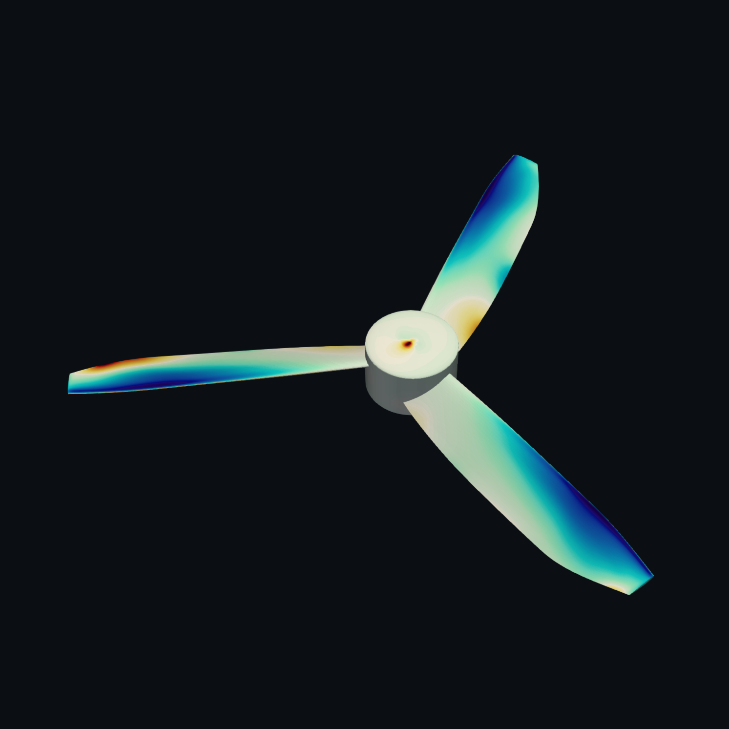
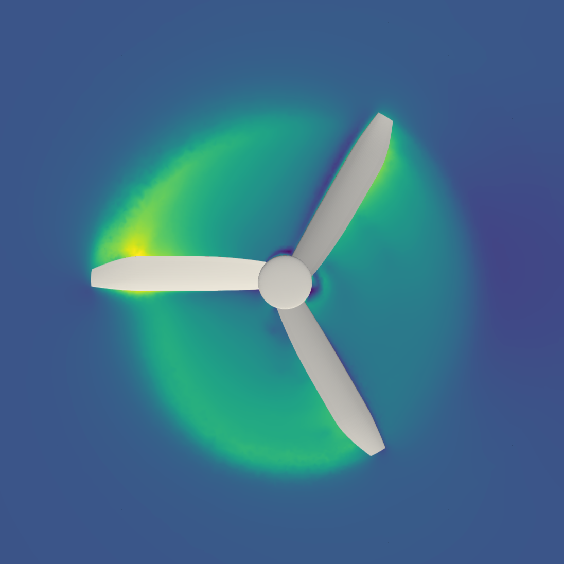
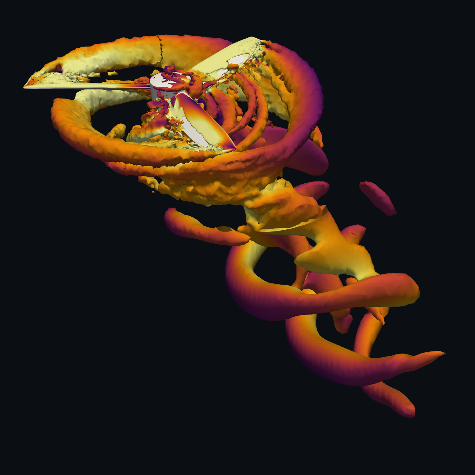
CFD RESULT: UNSTEADY CALCULATION
Key figures, flow fields and noise sources.
Thrust, torque and power are evaluated, together with the derived thrust and power coefficients and the efficiency or figure of merit. All key figures are set against the 1D prediction, so that the deviation is immediately visible.
The result viewer provides surface pressure (instantaneous and time-averaged), velocity fields in the mid-plane, the rotor plane and two wake sections, streamlines, blade tip vortices and acoustic sources as switchable layers in the browser.
The acoustic sources are estimated from the flow field as volume sources from the turbulence field according to Proudman. This shows where noise is generated. However, this evaluation does not replace a far-field prediction.
- KEY FIGURES
- T, Q, P, C_T, C_P, η / FoM
- DELIVERY
- Result viewer in the browser, technical report as PDF
Strength and vibration on the full model.
The structural analysis is carried out on the complete propeller based on the CAD model, fixed at both end faces of the hub. Bores are not modelled for the time being, and the hub is calculated as a solid body. A single blade with an equivalent clamping is deliberately not used, because the transition from the blade into the hub is precisely the critical zone.
Isotropic materials are calculated, currently PA6-GF30. A static structural analysis applies the centrifugal force at overspeed. The subsequent modal analysis of the loaded model yields the natural frequencies of the rotating propeller, which the Campbell diagram plots over rotational speed against the excitation orders. The reserves are stated separately for material and rotational speed. On request, the pressure distribution from the CFD is also applied as a load.
- LOAD CASES
- Overspeed (centrifugal force), modal analysis of the loaded model
- ON REQUEST
- CFD pressure loads, fatigue and service life
Limits of the methods.
A result is only as meaningful as the knowledge of its accuracy. The following limits are therefore also stated in every report.
- 1D DESIGNSweep, tip shape and installation effects (arms, fuselage, neighbouring rotors) are not taken into account. Cruise with a tilted rotor disc is an estimate and marked as such.
- AIRFOILSAt the lowest Reynolds numbers, the airfoil polar is the largest uncertainty in the chain.
- CFD STEADYReliable for axial inflow. In forward flight, however, the steady calculation is an approximation and the time-resolved calculation is recommended.
- TURBULENCEFully turbulent calculation; laminar–turbulent transition is not modelled.
- ACOUSTICSSource estimate and spectrum, no far-field measurement and no installation effects.
- STRUCTUREThe quick structural check in the 1D design is indicative; fatigue is only assessed in a separate analysis. The FEM currently covers isotropic materials; fibre composites on request.